Exploring the 2011 Massachusetts Travel Survey:
Barriers and Opportunities Influencing Mode Shift
Project Manager
Bill Kuttner
Project Principal
Annette Demchur
Project Contributor
Katie Pincus
Cartography
Ken Dumas
Cover Design
Kim DeLauri
The preparation of this document was supported
by the Federal Highway Administration through
MHD 3C PL contracts #32075 and #33101.
Central Transportation Planning Staff
Directed by the Boston Region Metropolitan
Planning Organization (MPO). The MPO is composed of
state and regional agencies and authorities, and
local governments.
The Boston Region Metropolitan Planning Organization (MPO) supports the Massachusetts Department of Transportation’s long-term objective of significantly increasing transit’s mode share. This increase in transit mode share is part of a larger goal of reducing the share of trips by single-occupant vehicles. Detailed travel data reported by participants in the 2011-Massachusetts Travel Survey (2011-MTS) have been analyzed in this study to inform the process of effecting the desired mode shifts.
The 2011-MTS contains information about all household travel, but it is especially detailed with respect to work trips and school trips. This study focuses on these two travel markets, defines relevant submarkets, and identifies aspects of key submarkets that make transit competitive. The characteristics of transit-competitive travel submarkets are quantified, and serve as a basis for discussing specific strategies to increase transit’s mode share.
The MPO has developed, and is constantly improving, a regional travel demand model, which intends to reliably predict changes in travel mode shares that result from demographic trends, infrastructure improvements, and certain types of policy initiatives. The mode choice variables incorporated in the regional travel demand model were estimated using data from the 2011-MTS; the last section of this study describes these variables and relates them to the mode shift analysis presented earlier in this study.
1.4 The Stated Preference Database
2.1 The Boston Region Commuting Market
2.2 Geographical Commuting Patterns
2.3 Mode Choice by Commuting Pattern
2.4 Transit-Competitive Commuting Patterns
3.1 The Basic Calculation: Dividing the Sample into Three Groups
3.2 Combined Influences of the Three Geographical Factors
4.1 Three General Strategies to Increase Transit Share
4.2 New Transit Services in Non-competitive Commuting Markets
4.3 Improved Service in Transit-Competitive Commuting Markets
4.4 More Commuters in Transit-Competitive Commuting Markets
4.5 Considering Commute Lengths
5.1 Identifying School Travel Markets
5.2 Primary School Travel Markets
5.3 High School Travel Markets
5.5 Opportunities to Influence Mode Shift
6.2 Mode Choice Model Coefficients
6.3 Opportunities to Influence Mode Shift
7.1 Review of the Work Trips Analysis Process
7.2 Mode-Shift Observations and Implications
7.3 Travel between Home and School
7.4 Regional Travel Demand Model
TABLE 1 ...... Boston Region Commuting Market
TABLE 2 ...... Mode Choice by Commuting Pattern
TABLE 4 ...... Commuting by Auto and Transit by Educational Attainment
TABLE 5 ...... Average Commute Distances in Miles
TABLE 6 ...... Distribution of Commuters and Commute Distances by Pattern
TABLE 7 ...... Boston Region MPO Area Students
TABLE 8 ...... Mode Shares in Primary School Travel Markets
TABLE 9 ...... Mode Shares by Household Vehicles in Primary School Travel Markets
TABLE 10 .... Mode Shares by Income in Primary School Central Sector Travel Market
TABLE 13 .... Elementary and Middle School Mode Shares by Travel Market
TABLE 14 .... Effect of Two-Mile Threshold on Elementary School Student Mode Shares
TABLE 16 .... Mode Shares in High School Travel Markets
TABLE 17 .... Mode Shares by Driver’s License Eligibility in High School Travel Markets
TABLE 18 .... Mode Share in College Travel Markets
TABLE 19 .... Mode Shares by College Type in Central Sector Travel Market
TABLE 20 .... Mode Shares by College Type Outside the Central Sector Travel Market
TABLE 21 .... Mode Shares by Income in Central Sector College Student Travel Market
FIGURE 1 .... Analysis Sectors
FIGURE 2 .... Transit Shares of 667,200 Transit-Competitive Commutes
FIGURE 3 .... Transit Shares for all Combinations of the Three Geographical Factors
In July 2014, the Boston Region Metropolitan Planning Organization (MPO) approved a work program for a study—Barriers and Opportunities Influencing Mode Shift. As originally envisioned in the MPO’s Unified Planning Work Program, this study was to have been completed in partnership with the Metropolitan Area Planning Council (MAPC). The MPO planned to conduct a statistical analysis using a variety of data sources to determine what factors have been the most important determinants of successful transit service. Using the same datasets, MAPC was to analyze the factors that influence mode shift for walking and biking. However, during the project scoping process, both MPO and MAPC staff realized that the analytical methodologies and datasets required for the transit analysis were very different than for walking and biking.
The changes needed to refocus the work were reflected in the work program for this study, the key findings of which are presented in this report. These findings will help to inform the MPO’s long-term objective of significantly increasing transit mode share while reducing single-occupant vehicle mode share.
The Massachusetts Travel Survey (2011-MTS), completed in 2011, was the central resource for this study. The 2011-MTS compiled responses from 15,040 Massachusetts households about the travel activity of household members. A summary of survey results is available at www.mass.gov/massdot/travelsurvey. Data from the 2011-MTS has already been used to calibrate the MPO’s new travel demand model. Travel demand models are used to predict how regional transportation systems likely would function in the future under various transportation-investment or demographic-trend scenarios.
In April 2014 the MPO released a study, Exploring the 2011 Massachusetts Travel Survey: Focus on Journeys to Work, which is available at http://bostonmpo.org/Drupal/exploring_2011_survey. The study organized data from the 2011-MTS and analyzed commuting patterns by travel modes. In a number of instances, this study made direct comparisons between the commuting patterns reported in 2011 with those cited in the prior household survey, completed in 1991.
The Barriers and Opportunities Influencing Mode Shift study moved beyond the Journeys to Work study by identifying factors that influence people to choose particular travel modes and relating those factors to policy issues, such as those that address how best to add new service where appropriate. The study team focused on work-commute data as the starting point for this study because of the significance of commuting distance on both the selection of residence location and mode choice decisions, and because of the availability of data.
The study team also obtained high-quality data for most types of school trips. Both work- and school-trip data were analyzed in the travel demand model to gain further insight into the factors affecting mode choice. While the 2011-MTS data are a key input to the travel demand model, the model also includes transportation system and geographic variables that represent characteristics of specific trips.
Most of the findings of this study were based upon geographical factors that affect commuting. Respondents to the 2011-MTS reported whether they worked, the location of their workplace, and their preferred commuting mode. The analysis began by dividing the sample of commuting workers into six groups based on the geographical patterns of their commutes. Then the mode shares were calculated for each group. Inspection of the mode shares in each group readily indicated that transit had an appreciable mode share among commuters with certain commuting patterns, which for the purposes of this study are referred to as transit-competitive commuting patterns.
The sample used to develop most of the findings about commuting in this study was selected in a two-step process. First, survey respondents whose commutes fell into one of three transit-competitive commuting patterns were selected. Second, commuters who either drive or choose to use transit were selected, forming the sample on which most of the analysis was based.
The sample commutes then were characterized based on whether the commuter had access to transit from home or work, and the availability of parking near the workplace. Both the availability of transit service near the origin or destination of a trip and scarcity of parking near the destination can encourage the use of transit. A goal of this study was to quantify the influence of proximity to transit and availability of parking on mode choice.
The responses of participants in the 2011-MTS were organized into several distinct tables:
This table contains information about the 15,040 participating households including home address, household income, and vehicle ownership.
This table presents information about the 37,023 individual members of the participating households, including whether they were employed or enrolled in a school, the location of their job or school, their preferred commuting mode, age, education level, and whether licensed to drive.
This file contains 190,215 records of places survey participants went to on the survey day. These data can be organized into trip segments, entire trips between activities, or journeys representing chains of trips. The table contains data from each household’s reporting day, during which all household members reported their locations and activities, and the means by which they reached each location.
The Journeys to Work study utilized the data from the Place Table, which was organized into chains of trips between primary residence and primary workplace. This allowed for a detailed analysis of how the journeys were structured, and reflected, for example, changes of mode, the presence of passengers, or the incidence of intermediate stops for activities on the way to work.
The Journeys to Work study found that a significant portion of employed respondents did not travel to their primary workplaces on the day of the survey for several common reasons. The average workweek is only 4.6 days, and many workers were scheduled to work on weekends and take their days off during the week. Vacation, sick days, occasional working from home, or traveling to a work-related location that is not the primary workplace were other reasons a worker may not have reported travel to the primary workplace on the survey day.
The 2011-MTS Person Table was used as the primary resource for this study. Because the survey respondents reported their preferred commuting modes regardless of whether they traveled to their primary workplaces on the survey day, the database used in this analysis is referred to as the Stated Preference database.
The sample of commuters in the Stated Preference database is somewhat larger than the sample that was analyzed in the Journeys to Work study for two reasons. First, the database contains responses from all commuters surveyed regardless of whether they traveled to work on the survey day. Because of the various causes listed above, only 79 percent of survey respondents who claim to commute to work actually traveled to work on the survey day. While this shortfall seems large, it was corroborated by analyzing data in the Household Table in the Journeys to Work study. Second, Massachusetts residents who live outside the region covered by the travel demand model and commute to jobs within the region were included in this analysis.
For this study, the original Person Table data was augmented with key data from the Household Table, such as the number of household vehicles. Transit access and demographic data developed using geographical information systems (GIS) techniques also were included, notably the coordinates of the nearest rail transit stops to home, workplace, and school.
Because the datasets used in the Journeys to Work study and this study were obtained and analyzed in two completely different ways, metrics such as mode shares calculated from these two sources were not expected to be identical. Some comparisons calculated on an aggregate basis were reassuringly close, and the two efforts should be viewed as complementary analyses of Boston’s regional commuting market.
The 37,023 individual respondents to the 2011-MTS represented approximately 0.59 percent of Massachusetts’ household population. The survey was designed so that each respondent represented a certain number of people in the overall population. This is referred to as a “weight factor”, and the average weight factor for each respondent was 170 (100/0.59). In surveys such as the 2011-MTS, weight factors vary widely among the various population groups sampled. Unless noted otherwise, all numeric values presented in this study are weighted survey responses.
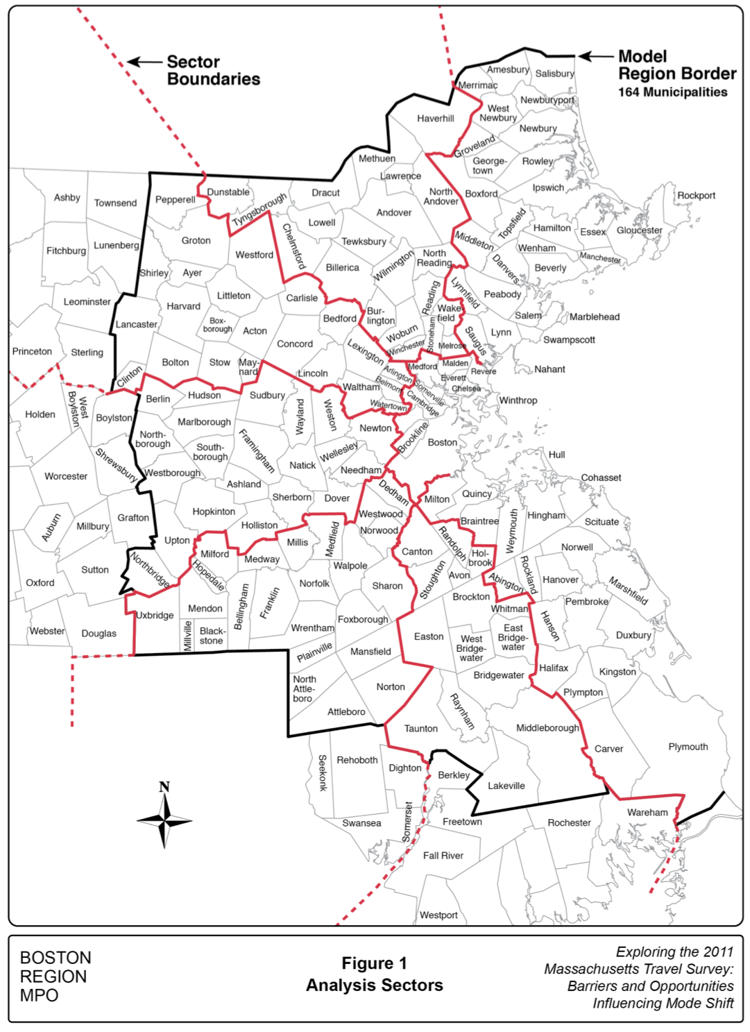
For this study, approximately one-third of Massachusetts residents were considered to be part of the Boston region commuting market, the composition of which is calculated in Table 1. The Boston region commuting market is organized around the 164 municipalities for which the Boston Region MPO travel demand model was developed, as shown in Figure 1.1 Approximately 101,000 residents in the model region commute to workplaces outside the model region and 133,100 workers from elsewhere in Massachusetts commute into the region. Both of these groups of commuters were considered part of the Boston region commuting market.
Ideally, about 130,000 commuters who travel into the region from Maine, New Hampshire, Rhode Island, and Connecticut also would have been included in this analysis as they clearly qualify as part of the Boston region commuting market. Unfortunately, no data about individual commuters were available from the Census’ 2006-2010 American Community Survey.
1 The travel demand model area includes the 101 communities of the Boston Region MPO plus 63 surrounding municipalities. The inclusion of these outer communities in the Boston Region MPO’s model provides significant analytical benefits. Model inputs throughout the model region are prepared to a uniform high standard.
Survey Subgroups |
Residents |
Massachusetts residents |
6,308,700 |
Residents in Boston region (164 municipalities) |
4,299,600 |
Resident who live and work in Boston region |
2,104,900 |
Residents who live in Boston region and work elsewhere |
101,100 |
Total Workers |
2,206,000 |
Residents who live elsewhere in Massachusetts and work in Boston region |
133,100 |
Total Boston region workers |
2,339,100 |
Home-centered workers |
221,900 |
Boston Region Commuting Market* |
2,117,200 |
* The Boston region commuting market does not include home-centered workers.
Numbers of residents and workers were calculated from the US Census and the 2011-MTS.
There were 221,900 workers, referred to as “home-centered,” who were not included in the Boston region commuting market. These workers either claimed that their primary workplace was at home, or reported a workplace location so far away that the mode choice was more appropriately thought of as a long-distance travel decision rather than a conventional commuting decision. Workers in the building trades and sales representatives, for example, need to travel, but they were considered home-centered.
For this study, it was assumed that respondents could commute between the model region and any location within Massachusetts. Workers living in the model region who reported their primary workplace as outside of Massachusetts were classified as “commuting” if their workplace was within 100 miles of their home, and as “home-centered” if greater than 100 miles.
In this study, the model region was divided into the same eight analysis sectors used in the Journeys to Work study: a central sector consisting of Boston and nine adjoining communities, and seven radial sectors. (See Figure 1.) The following six distinct commuting patterns were defined, based on type of sector-to-sector travel:
Both home and workplace are located within the central sector
Home is located in a radial sector and work is in the central sector
(includes residences outside of the model area)
Home is located in the central sector and work is in a radial sector
(includes workplaces outside of the model area)
Home is in a radial sector but work is in a non-adjacent radial sector
(one end of commute may be outside of the model area)
Both home and workplace are located within the same radial sector
Home is in a radial sector and work is in an adjacent radial sector
Mode shares varied greatly between the different commuting patterns, as shown in Table 2. For instance, driving was preferred by more than two-thirds of commuters, but this ranges from slightly more than half of the Radial commuters to fully 95 percent of the Adjacent Sector commuters. Central Area, Radial, and Reverse commutes were considered transit-competitive commuting options. The characteristics of transit-competitive commutes are discussed in detail in the following section.
Commuting Pattern |
All Modes |
Driving |
Transit |
No-auto |
Other |
Percent Transit |
|||
Central Area |
405,700 |
120,800 |
123,900 |
52,800 |
108,200 |
31 |
|||
Radial Commute |
354,100 |
181,500 |
152,100 |
4,300 |
16,200 |
43 |
|||
Reverse Commute |
103,100 |
79,300 |
9,600 |
8,500 |
5,700 |
9 |
|||
Distant Sector |
107,200 |
100,800 |
2,400 |
600 |
3,400 |
2 |
|||
Intra-Radial |
847,700 |
736,800 |
9,700 |
6,200 |
95,000 |
1 |
|||
Adjacent Sector |
299,400 |
284,200 |
2,400 |
1,300 |
11,500 |
1 |
|||
All Patterns |
2,117,200 |
1,503,400 |
300,100 |
73,700 |
240,000 |
14 |
|||
Transit-Competitive Commutes |
|
381,600 |
285,600 |
|
|
|
|||
Head-to-Head Mode Shares |
|
57% |
43% |
|
|
|
|||
|
|
|
|
|
|
|
|||
Total Transit-Competitive Commutes = 667,200 |
|
|
|
|
|
|
|||
Commuters who used transit were split into two groups. Commuters who used transit despite living in a household with an auto were considered as “choosing” transit and represented about 14 percent of all commuters. An additional four percent of commuters used transit but lived in households without an auto, and they were considered “no-auto transit” commuters. When combined, the total transit ridership share in this analysis closely matched the transit share calculated in the Journeys to Work study.
Walking, bicycle riding, using paratransit, and being given a ride all were grouped into “other modes” and made up 11 percent of commutes. Four percent of commuters reported that they were normally “given a ride,” but for the purposes of this analysis, they were not classified as choosing to drive.
The percent of commuters “choosing” transit for each commute pattern appears highest among commuters with the Central Area, Radial Commute, and Reverse Commute patterns, as shown in Table 2. While transit can be considered a competitive alternative to driving for those commuters, it is definitely not for those with the Distant Sector, Intra-Radial, and Adjacent Sector commuting patterns.
In this study, the competitiveness of transit was characterized by what is referred to here as the “head-to-head” mode share. This mode share is computed by ignoring all options except driving and choosing transit, and comparing these two choices. For instance, as shown in Table 2, 381,600 commuters drove to work in the three competitive submarkets and 285,600 chose transit—altogether, there were 667,200 transit-competitive commutes. Head-to-head against driving in these three submarkets, transit was used by 43 percent of commuters.
The six submarkets in Table 2 are listed in descending order based on how well transit competes against driving. While only 31 percent of commuters making Central Area commutes chose transit, it was the most popular mode for this pattern and exceeds the 30 percent of commuters who drive.
The traditional Radial Commute represents the largest mode share for transit, with 43 percent of commuters having chosen transit. Driving, however, tops transit with a 51 percent mode share. The other options were used by only six percent of commuters.
The third submarket where transit is considered competitive is the Reverse Commute, with nine percent of commuters having chosen transit. Largely, the Reverse and Radial Commute submarkets share the same transit infrastructure and transit competitiveness depends on suburban land-use patterns and transit-service schedules.
The three commuting patterns excluded from the transit-competitive sample were similar in that neither the commuter’s home nor workplace was in the central sector. Only about one percent of commuters chose transit in these situations. Only in the comparatively small submarket connecting distant sectors was the transit share as great as two percent. There are few transit options within radial sectors or between adjacent sectors, and the distant sector submarket is served to only a limited degree by the Red Line.
The 667,200 commuters who drove or chose transit in the three transit-competitive commuting submarkets made up about 32 percent of the commutes in the Boston region commuting market. The rest of this study examined these commutes as a group rather than considering the three patterns individually. Instead, the individual commutes in the sample were characterized by transit access and parking availability in order to measure aspects of a commute that make transit competitive.
The analysis of transit-competitive commutes began with a set of simple calculations. First, the sample of 667,200 transit-competitive trips was divided into three equal-sized groups of 222,400. Then the groups were examined in terms of three geographical metrics known to influence mode choice. For each metric, the transit mode share of the three groups was calculated.
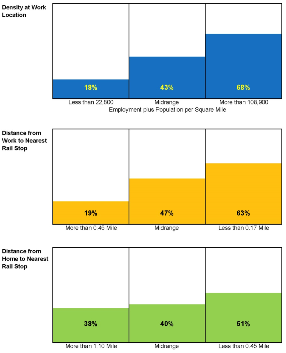
The calculations for three geographical metrics of interest are described below and shown in Figure 2.
Population and employment data for the traffic analysis zone of each workplace destination were summed and divided by the zone’s land area.2 This calculation provided a figure for combined population and employment density per square mile. All references to density in the analysis refer to this combined density. One-third of the commutes were to a workplace where the density was less than 22,800 people per square mile; and one-third of the destinations had a density that exceeded 108,900 people per square mile. The transit shares were 18 percent in the least dense group, 43 percent in the midrange group, and 68 percent in the densest group. Useful data for the regional parking supply was unavailable; thus density was used as a proxy for the level of demand for available parking.
One-third of commutes were to workplaces greater than 0.45 miles from a rail transit stop, and one-third were to workplaces within 0.17 miles of a rail transit stop. The transit shares were 19 percent in the most distant group, 47 percent in the midrange group, and 63 percent in the closest group.
One-third of commutes were from homes that were more than 1.10 miles from a rail transit stop and one-third were from homes within 0.45 miles of a rail transit stop. The transit shares were 38 percent in the most distant group, 40 percent in the midrange group, and 51 percent in the closest group. The 0.45-mile breakpoint defining groups for both workplace and home transit access is a coincidence.
For purposes of this study, the distance to a rail transit stop was considered an appropriate index of access to transit. While many homes and workplaces are closer to a bus stop than to a rail transit stop, rail transit represents a connection to destinations throughout the regional commuting market. Furthermore, many bus routes serve commuter rail and rapid transit stations, and a location being close to a rail transit station often implies that it is close to a number of bus stops as well.
This initial analysis clearly illustrated the relative importance of these geographic factors in mode choice. Density near the workplace, and by implication high demand for parking, most strongly reflects the competitive strength of transit. The distance between the workplace and a rail transit stop determines the attractiveness of transit only slightly less. Historically, early rail and transit corridors served the employment concentrations of the time; since then a significant portion of subsequent job growth reinforced this pattern.
In contrast, proximity of a residence to transit increased transit competitiveness to a much smaller degree. This sample included only households with an available auto. Using an auto to reach a convenient transit stop counted as choosing transit, as transit stops farther away than the typical walking distance can still be attractive points at which to enter the transit system. The drive-access transit commuter arrives at work without the car, and the final walk distance to the work site remains an important factor.
2 Traffic analysis zones (TAZs) are relatively small geographic units used in transportation planning, especially for travel demand model development.
The choices of individual commuters may be seen even more clearly if all three geographic factors are used to characterize transit-competitive commutes. While variation in density at the work location most closely tracks the variation in transit mode share, a wide range of transit shares may be observed within these three groups based on transit access at both the work and home ends of the commute.
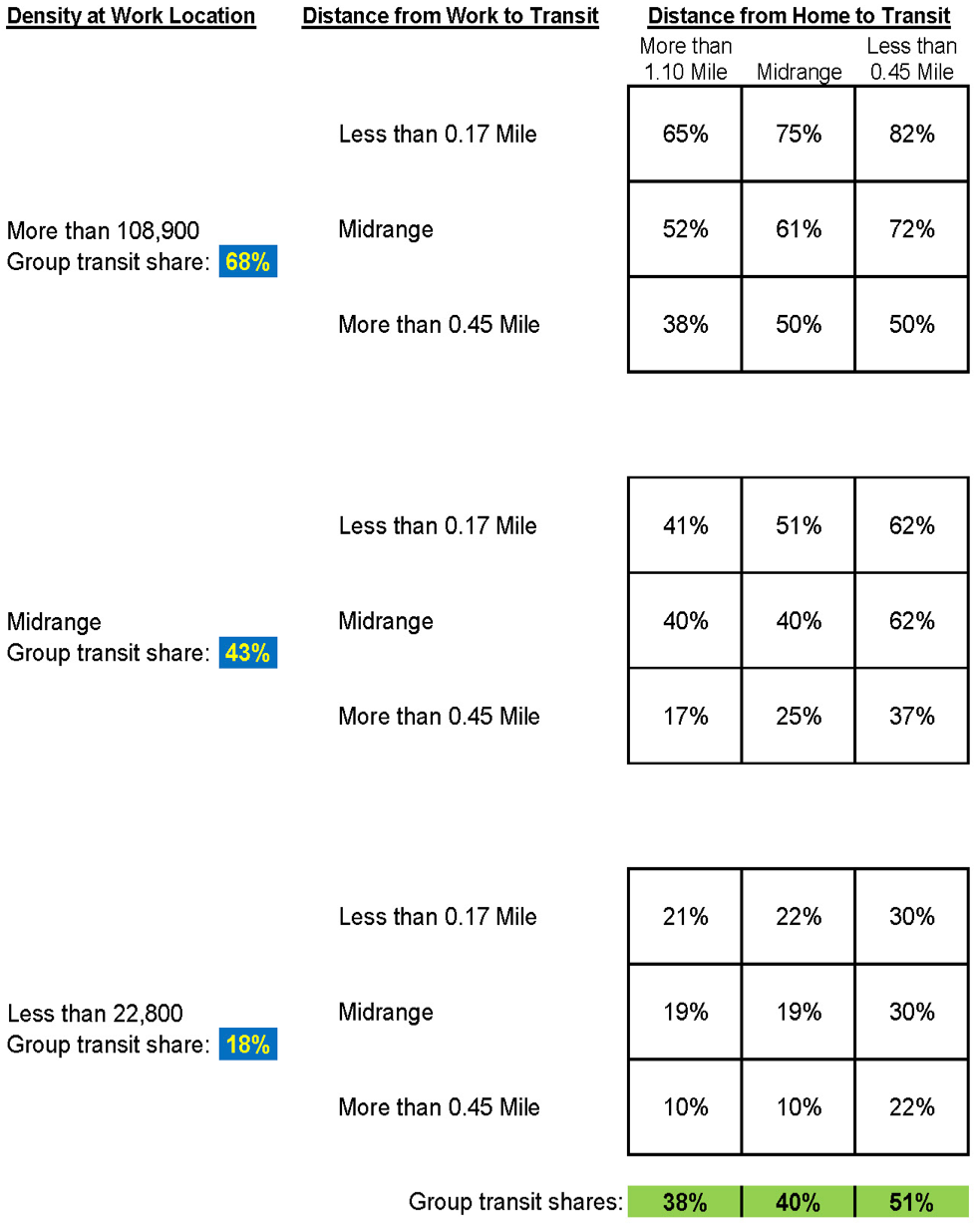
Figure 3 shows transit mode shares based on these geographical factors. The data were organized first based on the density at the work destinations, then subdivided based on the distance to transit from the commuter’s home and workplace. The commutes into the densest work locations, as a whole, had a 68 percent transit share; however, transit shares varied considerably based on the combined factors of commuters’ distance to transit from work and home.
Transit mode shares ranged in the densest group from 38 percent for commuters most distant from transit at both the home and work ends of their commutes to 82 percent for commuters closest to transit at both ends of the commute. Similarly, workplaces in midrange density areas had an average transit share of 43 percent, but this in turn ranged from a low of 17 percent up to 62 percent depending on transit access at the commute ends.
The transit share ranged from only 10-30 percent for the least-dense employment locations, with a group-wide average of 18 percent. This indicates that if parking is plentiful, driving remains a popular mode even if proximity to transit services is good at both ends of the commute.
These data also may be viewed from the perspective of the distance from home to transit. As shown in Figure 3, commuters who live closest to transit had a transit share of 51 percent, but this ranged from a low of 22 percent in low-density areas to 82 percent in high-density areas. Of commuters who live farthest from transit—in households that have an auto available that might be used for transit access—38 percent chose transit. The wide range of possible transit shares for this group—10-to-65 percent—was correlated with the work location density and transit access.
Another pattern is noticeable in Figure 3. The upper-right corner of each major rectangle represents close transit access at both ends of the commute. The lower-left corner represents distant transit access at both ends. However, moving from cells in the upper left to cells in the lower right implies trading transit proximity to work for transit proximity to home. Similarity of transit shares across these diagonal values perhaps implies a tolerance for the total amount of walking, with commuters considering walks at both the home and work ends of the commute as they make their mode choice. (This observation would not apply to commuters driving to transit.)
The findings and recommendations of this study are based primarily on detailed geographical data incorporated into the Stated Preference database. These geographically based analyses inform strategies that may increase transit’s share of regional travel. However, the Stated Preference database also offers detailed information about survey respondents that can indicate whether travel markets could be targeted on a socio-economic basis.
Table 3 shows the transit shares of competitive commutes for surveyed households with various income levels. Seven household income levels are defined in the table; transit shares vary within a tight range in these subgroups, from 41-45 percent, averaging 43 percent. No relation between transit share and income is noticeable with casual inspection. A reasonable conclusion from the data in Table 3 is that if the transit mode share increases within a geographical submarket, new commuters from all income levels would be included based on their presence in the particular submarket.
Annual Household Income |
Auto Commuters |
Transit Commuters |
Combined |
Percent Auto Share |
Percent Transit Share |
$150,000 or greater |
110,200 |
78,400 |
188,600 |
58 |
42 |
$100,000 - $149,999 |
72,300 |
60,300 |
132,600 |
55 |
45 |
$75,000 - $99,999 |
69,300 |
50,200 |
119,500 |
58 |
42 |
$50,000 - $74,999 |
68,400 |
50,800 |
119,200 |
57 |
43 |
$35,000 - $49,999 |
31,200 |
24,200 |
55,400 |
56 |
44 |
$25,000 - $34,999 |
15,200 |
11,200 |
26,400 |
58 |
42 |
Less than $25,000 |
15,000 |
10,500 |
25,500 |
59 |
41 |
All Incomes |
381,600 |
285,600 |
667,200 |
57 |
43 |
Transit-competitive commutes also may be categorized by education level, as shown in Table 4. Unlike household income, level of education is an attribute of the individual commuter. Eighty-eight percent of transit-competitive commuters have some education beyond high school; 42 percent of those with an undergraduate degree and 45 percent of those with a postgraduate degree chose transit. Transit is used by 38 percent of the smaller group of commuters without any college education. This smaller transit share may reflect the location of employment opportunities, such as large auto-oriented shopping centers, for this demographic segment. Commuting preferences are consistent enough acro-ss levels of education that, as in the case of income, no submarket appears as a clear market opportunity for transit.
Education Level |
Auto |
Transit |
Combined |
Percent Auto |
Percent Transit Share |
Postgraduate degree |
145,600 |
119,100 |
264,700 |
55 |
45 |
Undergraduate study |
185,500 |
135,900 |
321,400 |
58 |
42 |
High school or less |
50,500 |
30,600 |
81,100 |
62 |
38 |
All Education Levels |
381,600 |
285,600 |
667,200 |
57 |
43 |
This section presents three general strategies for increasing the transit share of commuting trips among the Boston region commuting market, and discusses implications of the findings presented in prior sections 2 and 3 for each of the three strategies. These strategies address aspects of the six commuting submarkets presented in Table 2:
The Distant Sector, Intra-Radial, and Adjacent Sector commutes are not considered transit-competitive. New services could be introduced to serve these commuting submarkets.
The head-to-head mode share calculation showed that transit is preferred by 43 percent of commuters, instead of driving, in the commuting submarkets where transit is relatively strong: Central Area, Radial Commute, and Reverse Commute. Expanded or improved services could increase transit’s share in the submarkets where it shows strength today.
If long-term demographic and economic growth adds commuters in areas where transit is strong, the overall share of transit commutes will also increase, if there is available capacity on the system.
When considering these commuting strategies, a key characteristic works in the planner’s favor: almost all elements of the regional transportation system serve more than one of the commuting submarkets. The commute of any individual survey respondent may be characterized as fitting into one of the commuting patterns, but any lane of traffic or any transit vehicle will contain commuters from several of the submarkets.
Another common characteristic of these strategies complicates the efforts to influence mode choice. Planners and operating agencies are in a good position to focus on one end of a commute. If a new transit service or expressway interchange is being considered, homes and workplaces convenient to the envisioned improvement can be known and future growth can be predicted and planned for. However, the other end of each trip that will define the commuting pattern will be located throughout the region and can only be estimated.
Among the six commuting patterns in Table 2, transit was only competitive if at least one end of the trip was in the central sector. Of the 1,254,300 commuters in the Distant Sector, Intra-Radial, or Adjacent Sector submarkets, 89.2 percent chose to drive compared with only 1.2 percent who chose transit. Of the remaining commuters, 4.4 percent were given a ride, 3.0 percent walked, 0.8 percent bicycled, and 0.5 percent used a taxi or van shuttle. Another 9,100 commuters in these three submarkets were transit users without autos; they represented 0.6 percent of commuters.
The Intra-Radial commutes were by far the largest of the six commuting submarkets. Of the region’s 1,503,400 commuters that drove, almost half (736,800) commuted within the same radial sector. Transit services available to the 9,700 commuters that chose transit in this submarket are limited. Local bus services are offered in a number of the region’s older cities, but these vary in coverage and hours of operation. The commuter rail system also can be used between stations in the same radial sector. Approximately 16,000 commuters did use transit to make an Intra-Radial commute, but 6,200 of them lived in households without an auto.
The survey analysis indicates several implications for efforts to expand transit share in the Intra-Radial submarket. First, the willingness of commuters to choose transit depends on conditions at both ends of their commute. A new transit service directly adjacent to a residential complex would win ridership based on the geographical characteristics at the work end of the commute. As shown in Figure 3, the head-to-head probability might range from 22 percent to 82 percent depending on conditions at the workplace. If density at the workplace is low, implying relative ease of parking, the probability of choosing transit might be only 30 percent even if the service happens to run near a commuter’s workplace.
Another implication concerns the small number of transit riders in this submarket. The head-to-head transit share for all six commuting patterns combined is only 16.6 percent. Even if the number of Intra-Radial commuters choosing transit doubled, moving another 9,700 commuters from auto to transit, the region-wide head-to-head transit share would increase to only 17.2 percent.
A third implication is actually somewhat more optimistic. Transit service expansions or improvements implemented within a radial sector, in all likelihood, would improve conventional Radial and Reverse Commutes, submarkets where transit is already competitive. Most suburban transit authorities operate bus routes that connect with commuter rail service at one or more points. While few commuters transfer between bus and rail today, improved bus services that succeed in attracting new Intra-Radial commuters also might develop some connecting ridership, using both commuter rail and local bus for Radial and Reverse Commutes. While the new ridership in each submarket might be small, the combined increases from all improved submarkets could justify the transit service improvement.
The same implications would apply to efforts to expand transit share in the smallest non-competitive commuting submarket, Distant Sector commutes to non-adjacent sectors. Of the 1,254,300 non-transit-competitive commutes, only nine percent (107,200 commutes) were the often-problematic commutes between homes and workplaces in non-adjacent sectors. Even with auto-dependent suburban lifestyles, the vast majority of workers have managed to arrange for homes and jobs roughly on the same side of downtown Boston.
Transit usage is higher in this small submarket than in the Intra-Radial submarket, with 2,400 Distant Sector commuters having chosen transit, which represents a head-to-head mode share of 2.3 percent. The transit network does connect non-adjacent sectors, but usually requires multiple transfers, which is an unpopular hassle for commuters.
One proposal to better serve this commuting submarket is a North Station-South Station rail link, which could offer through-routed commuter rail service and reduce the required transfers between some of the more distant non-adjacent sectors. The North-South Rail Link has not yet been evaluated at this level of detail, but if a project of this scale were to quintuple transit use in this submarket to 12,000, the increase of 9,600 would be comparable to the increase described above from doubling the Intra-Radial transit commutes, and would move the transit share from 16.6 to 17.2 percent. The issue here is that the submarket is simply small. Furthermore, realizing any mode shift would depend upon conditions at both ends of the commutes.
However, this kind of service improvement also would improve service in the Central Area, Radial, and Reverse Commute submarkets where transit is already competitive. Even if improving the transit share of Distant Sector commutes were a planning priority, the value of this kind of investment would depend largely on how much it would increase the transit share in the submarkets where transit already is strong.
The survey-based implications presented in the previous section also are valid when considering competition in transit’s strong submarkets. Potential growth within a submarket is related to the size of the submarket. Mode choice depends on circumstances at both ends of the commuter’s trip. New transit ridership resulting from an improvement may be spread across several submarkets, both weak and strong.
In the transit-competitive submarkets, there is a fourth important implication: transit mode share can decrease as well as increase. Where the transit share is negligible, the worst outcome of expanding transit service is committing scarce financial resources while winning few new commuters. Where transit usage is strong, there is always a danger that actions by an operating agency or events beyond its control, such as weather, may make taking transit a less attractive choice. Conversely, driving may become more attractive because of low fuel prices. These types of circumstances have the potential to change the competitive equilibrium meaningfully.
Once again, the 9,700 Intra-Radial commuters who chose transit can serve as a benchmark. A 3.4 percent increase or decrease in transit use in the transit-competitive commuting submarkets would equal the number of commuters who chose transit in the Intra-Radial submarket. A 3.4 percent change in transit commuters in transit’s strong markets is still substantial and likely would not be an outcome of changing gas prices or memories of recent bad commutes. In addition, while the economy can change transit ridership, it is less likely to change transit’s mode share because expansion or contraction of the regional job market is across all modes and commuting markets.
The expansion and improvement of transit services in transit’s strong submarkets will increase transit’s mode share because of the favorable conditions in terms of density and proximity to transit. For example, the Green Line Extension in Somerville will make available a speedier service with fewer transfers to the large number of commuters who reside or work in Somerville. Somerville is in the central sector and all commutes to or from endpoints in Somerville will be in transit’s strong Central Area, Radial, or Reverse Commute submarkets.
A commuter traveling into or out of Somerville today may drive because the distance to transit at the Somerville end of their commute is 0.6 miles, while he or she is only willing to walk 0.5 miles to use the existing service. With the improvements to transit associated with the Green Line Extension, a 0.6 mile walk may become acceptable. However, it will only be an acceptable walk if the other end of the commute is also considered acceptable for choosing transit.
Conversely, if the reliability or frequency of transit service gradually deteriorates, then transit share will decline with the loss of customers whose commutes are near the limit of their willingness to walk. A commuter who was willing to choose transit when the walk at one end of the commute was less than 0.5 miles may be willing to stay with transit. However, if a service is completely eliminated and the walk to transit increases dramatically, a large number of commuters may choose to drive even if their willingness to walk has not changed.
The available data used for this analysis gives some idea of the size and location of the commuting markets in which transit has achieved its most advantageous competitive equilibrium. At this level of analysis, it is only possible to speculate about the scale of market share increases that could be achieved through specific improvements to transit service. The most practical strategy might be to implement a number of small but measurable transit improvements. This would need to be accompanied by sustained efforts to protect transit’s existing market by avoiding any material decline in service.
A third general strategy is to increase the total amount of commuting that takes place in the three competitive transit submarkets. The high level of auto-dependency in commuting has long been attributed to patterns of urban and suburban development. We hope that with a better understanding and appreciation of commuting patterns and impacts, development may be guided to facilitate the use of transit, or at least not encourage driving.
The findings of this study speak directly to this topic. Municipal authorities can encourage employment and residential development convenient to transit, setting the conditions for transit commuting growth. However, as shown in Figure 3, the choice of commuting mode depends on conditions at both ends of the commute, even in the transit-competitive submarkets.
Workers in the region’s highly mobile labor force will choose the workplace that best matches their career aspirations. Commuting convenience may enter into that calculation as a “tie breaker,” but few people will accept what they consider an inferior job simply based on the commute. Only modes connecting with the preferred job location will be part of the choice set, no matter how carefully the built environment is crafted.
The term “transit-oriented development” is most frequently used to describe development programs seeking to take advantage of high-quality transit service in areas viewed at the time as highly auto-dependent. Of course, new developments in an urban core that is well-served by transit are also “transit oriented.” New development in either of these situations creates conditions for transit growth in several respects, even if the amount of growth depends on factors that developers and planners can only estimate.
First, workers in households with a car may be amenable to choosing transit simply because one end of the commute is convenient to transit. In many cases, transit access may also be good, or at least adequate, for all of a household’s travel. Households in this situation may forgo owning a car altogether, even if the household income can support car ownership.
As shown in Table 2, the 2011-MTS reported a substantial amount of commuting in the “No-auto Transit” category. Many commuters in this category may not be able to drive or afford a car. While “No-auto Transit” commuters could not be subdivided on this basis using the 2011-MTS, both of these subgroups can be attracted to convenient transit-oriented developments.
Finally, a number of communities and permitting authorities make encouragement of non-auto travel a condition for new developments, both urban and suburban. If attractive transit services are available, either existing or new, these policies can aspire to ambitious transit-use objectives. Absent useful transit offerings serving important travel markets, however, these efforts may not rise above symbolic.
Where economic and development trends are adding commuters in transit’s strong markets, the transit system can take advantage of these trends simply by maintaining its service offering at a competitive level. If service deteriorates or contracts, competitive ridership losses could offset these positive trends.
Expanding the transit system can strengthen positive economic and development trends, adding commuters in transit’s stronger markets. Earlier periods of public transportation expansion were investor-supported and were anticipated to generate profit as a return on capital investments. Investors and lenders calculated the mutual reinforcement of transit infrastructure, real estate development, and ridership to make numerous transit and urban real estate investments profitable. While public transportation is no longer expected to be profitable, synergies between transit infrastructure and development trends still exist and should be considered as part of any plan to increase transit’s share of regional travel.
The focus of this analysis so far has been to identify and measure geographical characteristics of commutes that influence mode choice. Circumstances at the ends of commutes such as transit access and density clearly relate to commuter behavior. In contrast, the length of the entire commuting distance from residence to workplace does not appear to correlate with the choice of mode.
Table 5 shows the average commuting distances for regional commuters who drove or chose transit. There is large variation in commuting distances across the six commuting patterns, but the distances for driving and transit are similar for most commuting patterns.
Commuting Pattern |
Driving |
Transit |
Combined |
Central Area |
3.1 |
3.6 |
3.3 |
Radial Commute |
16.0 |
16.3 |
16.2 |
Reverse Commute |
13.5 |
9.9 |
13.1 |
Distant Sector |
27.1 |
29.9 |
27.2 |
Intra-Radial |
6.9 |
6.5 |
6.9 |
Adjacent Sector |
15.1 |
13.1 |
15.1 |
All Patterns |
11.0 |
10.6 |
10.9 |
Competitive Commutes |
11.4 |
10.6 |
11.1 |
The one submarket where total commuting distance differed between these two modes was the Reverse Commute, where the average reverse commute by transit was several miles shorter. Reverse commuters using transit need to travel to suburban workplaces convenient to transit, and these locations are, on average, closer to the central sector than is the suburban job market as a whole. The importance of workplace proximity to transit was calculated directly in Figures 2 and 3. In contrast, Radial commutes were virtually the same distance for both modes since radial commuters had the option of driving to transit stops.
There are, however, policy implications associated with commuting distances. Efforts, both successful and unsuccessful, to preserve and expand the transit share of commuting trips will have impacts on the region’s transportation system by changing traffic congestion, greenhouse gas emissions, and transit vehicle utilization. By looking at the distribution of commuting miles by commute pattern, it is possible to anticipate these impacts and optimize mode-shift strategies.
In Table 6, the 1,803,500 commuters who either drove or chose transit—the head-to-head battleground of this analysis—have been distributed into the six commuting patterns both in terms of the number of commutes and the total commuting distances between residences and workplaces.
Commuting Pattern |
Average Distance (miles) |
Commutes |
Percent of Total |
Total Distance (miles) |
Percent of Total |
|
Central Area |
3.35 |
244,700 |
14 |
820,000 |
4 |
|
Radial Commute |
16.16 |
333,600 |
18 |
5,391,000 |
27 |
|
Reverse Commute |
13.10 |
88,900 |
5 |
1,165,000 |
6 |
|
Distant Sector |
27.22 |
103,200 |
6 |
2,809,000 |
14 |
|
Intra-Radial |
6.88 |
746,500 |
41 |
5,136,000 |
26 |
|
Adjacent Sector |
15.13 |
286,600 |
16 |
4,336,000 |
22 |
|
All Patterns |
10.90 |
1,803,500 |
100 |
19,657,000 |
100 |
|
Transit-Competitive Commutes |
11.06 |
667,200 |
37 |
7,376,000 |
38 |
|
Note: The total distance for each commuting pattern was calculated by multiplying the average distance times the number of commutes.
The 667,200 commutes in the Central Area, Radial and Reverse Commute submarkets are considered transit-competitive and they make up 37 percent of the total commutes. Similarly, these three submarkets account for 38 percent of the total miles commuted.
The individual submarkets, however, showed much greater differences between the shares of commutes and the shares of miles traveled. Transit was most competitive in the Central Area submarket, with more people choosing transit than driving. However, as the average trip length in this submarket was only 3.35 miles, the 14 percent of commutes represents only four percent of the miles traveled. Given that conventional radial commuting made up 18 percent of these commutes, but 27 percent of the head-to-head commuting miles, it is understandable why so much emphasis is put on serving this commuting submarket.
As mentioned earlier, the largest commuting submarket consisted of Intra-Radial commutes, which made up 41 percent of the total commutes. The Intra-Radial commuters are not well served by transit. Even with a below-average commuting distance, these commutes still made up 26 percent of the commuting miles. While there were almost as many Intra-Radial as Radial commuting miles, the travel volumes for the Intra-Radial commutes were not aligned in corridors, which poses a challenge for providing service cost effectively. If strategies to shift drivers to transit were most successful for the shorter commutes in this submarket, the overall impact could be limited.
The lengthy Distant Sector commutes present a distinct contrast. Only six percent of commuters had this type of commute, but taken together these commutes make up 14 percent of commuting miles. This disproportionate level of roadway usage helps explain ongoing interest in developing cost-effective suburb-to-suburb transit strategies.
The relevant distances influencing mode choice are those between residences and workplaces with their respective transit services. End-to-end commute distances help give a more complete picture of regional commuting than mode choice alone and can be useful in informing mode-shift strategies.
The 2011-MTS asked whether each respondent was enrolled in school, and those who answered yes were considered students for the purpose of this study.3 Respondents who were enrolled in school also were asked their education level, which ranged from preschool to graduate school, and the typical mode they used to commute to school. In order to focus on opportunities for mode shift within the Boston Region MPO area, only students who attended school in the region, or who lived in the region and attended school elsewhere in Massachusetts, were included in this analysis.
The study team defined major school-travel markets within the Boston Region MPO area by education level and geographic location of the school. Several factors that influence mode choice, such as student age, school schedule, and availability of school-provided transportation, vary significantly by education level. For example, primary school students, who generally have relatively short commutes, might rely on their parents to make their mode choices, and likely would not use transit on their own. Some high school students have the option to drive, while college students may choose where to live based on the locations of their schools.
The regional travel demand model classifies school trips as primary school (K-8 grades), high school (9-12 grades), college commuter, and college resident. Survey responses were categorized using these classifications to be consistent with the model. The household survey was not administered to college students living in campus housing such as dormitories, so all of the college-level students who responded to the survey were assumed to be in the college commuter category. This category encompasses all of the higher education responses in the survey: technical/vocational school, community college (two-year college), university (or four-year college), and graduate school (or professional).
Table 7 shows the household population of students for each of the education-level categories in this analysis. The survey responses were expanded using weighting factors from the 2011-MTS to reach totals that represented the census population. Home-schooled students were not included because they did not travel to attend school. Respondents who did not know their modes or refused to answer the question also were excluded.
3 The survey requested that adults in households with children younger than 14 years old report the travel of those children for them. This study refers to those children as “respondents” for simplicity.
Survey Subgroups |
Primary School Students |
High School Students |
College Students |
All Students |
Students who reside and go to school in MPO area |
357,850 |
178,302 |
179,310 |
715,4622 |
Students who reside in MPO area and go to school elsewhere in Massachusetts |
3,632 |
3,411 |
12,785 |
19,8288 |
Total students who reside in MPO area |
361,482 |
181,713 |
192,095 |
735,2900 |
Students who go to school in MPO area and reside elsewhere in Massachusetts |
13,679 |
10,284 |
34,805 |
58,7688 |
Total students who reside and/or go to school in MPO area |
375,161 |
191,997 |
226,900 |
794,0588 |
Home-centered students |
5,108 |
1,221 |
13,919 |
20,2488 |
Students who did not respond to survey |
1,468 |
779 |
3,543 |
5,7900 |
Total students excluded from study |
6,576 |
2,000 |
17,462 |
26,0388 |
Total students included in the study* |
368,585 |
189,997 |
209,438 |
768,0200 |
* Total students excluding home-centered students and students who did not respond to the survey
As shown in Table 7, more than half of the student population is in primary school, and there are more college students than high school students. Most students at all education levels who either live in or attend school in the Boston Region MPO area have a commute that occurs entirely within the MPO area as well. Compared to primary school and high school students, a larger percentage of college students attend school in the MPO area and live outside the region. Primary and high schools typically serve students who live in close proximity, while colleges attract students from farther distances based on their specialties.
The major school-travel markets were further defined based on the geographic locations of the schools. Schools in the central sector are located within a much denser transit network than schools in the rest of the MPO area. This affects the likelihood of transit being a feasible mode choice. Within each education level category, students attending schools located in the central sector were treated as a separate travel market because of this major factor affecting mode choice.
Survey respondents who indicated that they were enrolled in school were asked to specify their usual means of travel to school from 14 options, including 11 transportation modes. The transportation modes were grouped into the following for analysis: bike, drive, (auto) ride, school bus, transit, walk, and other (including taxi and paratransit). The remaining options were being home-schooled, not knowing their mode, and refusing to answer the question. Students who selected the latter three responses were not included in the mode-choice analysis. The mode shares for the primary school travel markets are shown in Table 8.
Mode |
Students in |
Students Elsewhere |
Percent Share |
Percent Share |
Bike |
3,307 |
2,347 |
3 |
1 |
Drive |
0 |
0 |
0 |
0 |
Other |
0 |
177 |
0 |
0 |
Ride |
33,397 |
91,702 |
30 |
36 |
School bus |
35,046 |
113,204 |
32 |
44 |
Transit |
9,467 |
4,770 |
9 |
2 |
Walk |
29,631 |
45,537 |
27 |
18 |
Total |
110,848 |
257,737 |
100 |
100 |
As shown in Table 8, the ride mode share was 30 percent for students attending school in the central sector and 36 percent for students attending school elsewhere in the region. Because primary school students cannot drive, getting a ride was the only auto-based mode in these travel markets. The survey results did not provide information about whether these students got rides as part of trips their parents already would make, such as driving to work. Either way, it is desirable to shift these auto-related trips to transit or, more realistically, the school bus, walk, and bike modes.
The share of primary school students who took transit was larger in the central sector travel market than elsewhere in the region. However, the transit mode share in the central sector was still relatively low at nine percent, which reflects the young age of primary school students. Fewer students rode a school bus in the central sector than outside the core area. This was probably a result of the greater population density and better walkability in the central sector. Walking had a larger mode share in the central sector than outside the core area as well.
The mode choice for primary school students or their parents is not as simple as deciding between auto and transit. Table 8 shows that the ride, school bus, and walk modes were all competitive in both primary school travel markets. Although transit is not competitive in these markets, opportunities may exist to shift some of the share from ride to the other competitive modes. This subsection analyzes the impact of various factors on mode share in each travel market to identify opportunities to influence mode choice in these markets.
The number of vehicles in a household had a clear effect on certain mode shares. For example, the ride mode share was significantly smaller in households without a vehicle than in households with at least one vehicle, as students in households without vehicles would rely on members of other households to pick them up for school. The changes in the shares of the other modes are more nuanced, but provide valuable information about the behavior of students in zero-vehicle households.
Table 9 shows the mode shares for households without a vehicle and households with at least one vehicle in each of the primary school travel markets. As expected, the transit and school bus mode shares were smaller in households with at least one vehicle than in households with no vehicles in both markets. However, in the central sector the walk mode share was greater for students in households with vehicles than for students in households without vehicles. This may reflect fewer transit options in neighborhoods with higher rates of auto ownership.
The mode shares were similar between the central sector and elsewhere, except the school bus and walk mode shares for households with a vehicle. The school bus mode share was much smaller and the walk mode share was larger in the central sector than elsewhere in the region. This may reflect the difference in density between the two travel markets. It is also interesting to note that the transit mode share was similar for households without a vehicle in both travel markets.
Mode |
Percent |
Percent Households |
Percent Zero-vehicle Households Elsewhere |
Percent |
Bike |
3 |
3 |
0 |
1 |
Other |
0 |
0 |
0 |
0 |
Ride |
6 |
38 |
3 |
36 |
School bus |
52 |
25 |
58 |
44 |
Transit |
18 |
6 |
17 |
2 |
Walk |
21 |
28 |
21 |
18 |
Total |
100 |
100 |
100 |
100 |
Because of the different costs of the transportation modes, household income was considered as a factor affecting mode choice. Table 10 shows the mode shares by income bracket for the central sector primary school travel market. No significant trends were observed in the mode shares by income bracket for students attending school elsewhere in the region, so those mode shares are not included here.
Table 10 shows that the ride mode share generally increased as income increased, while the school bus mode share generally decreased. Furthermore, the school bus mode share was larger than the ride mode share for the lower income brackets, while the ride mode share was larger than the school bus mode share for the higher income brackets. These trends may reflect the impact of the cost of vehicle ownership and usage on mode choice in the central sector.
Household Income |
Percent Ride |
Percent School Bus |
Percent Transit |
Percent Walk |
Less than $25,000 |
11 |
47 |
16 |
24 |
$25,000 - $34,999 |
31 |
48 |
6 |
16 |
$35,000 - $49,999 |
18 |
36 |
9 |
36 |
$50,000 - $74,999 |
36 |
40 |
3 |
14 |
$75,000 - $99,999 |
57 |
10 |
8 |
21 |
$100,000 - $149,999 |
51 |
12 |
5 |
27 |
$150,000 or greater |
30 |
17 |
5 |
45 |
Note: Bike and other mode shares are not shown because they are very small.
The distance between home and school had an effect on mode choice in both primary school travel markets. Table 11 shows the mode shares by distance between home and school for the central sector primary school travel market. Table 12 shows the mode shares for the non-central sector travel market.
In the central sector, the ride and school bus mode shares did not appear to be correlated with the distance between home and school. The school bus mode share was notably low at 18 percent for distances within one mile. For the same distance, almost half of the students walked to school. This is reasonable given the short distance and the school bus policy, which is explained in the next subsection.
Distance between Home |
Percent Ride |
Percent School Bus |
Percent Transit |
Percent Walk |
Less than or equal to 1.00 |
27 |
18 |
6 |
46 |
1.01 - 2.00 |
38 |
52 |
5 |
0 |
2.01 - 3.00 |
35 |
40 |
21 |
4 |
3.01 - 4.00 |
30 |
49 |
21 |
0 |
4.01 - 5.00 |
26 |
63 |
11 |
0 |
Greater than 5.00 |
37 |
48 |
14 |
1 |
Note: Bike and other mode shares are not shown because they are very small.
Distance between Home |
Percent Ride |
Percent School Bus |
Percent Transit |
PercentWalk |
Less than or equal to 1.00 |
37 |
27 |
1 |
33 |
1.01 - 2.00 |
26 |
71 |
1 |
2 |
2.01 - 3.00 |
26 |
73 |
1 |
0 |
3.01 - 4.00 |
34 |
61 |
5 |
0 |
4.01 - 5.00 |
46 |
49 |
2 |
3 |
Greater than 5.00 |
67 |
23 |
7 |
3 |
Note: Bike and other mode shares are not shown because they are very small.
Outside the central sector, the school bus mode share was larger than the ride mode share for distances between one and five miles. The ride mode share was larger than the school bus mode for the shortest and longest trips from home to school. One-third of students living within one mile of school walked, which is less than the walk mode share in the central sector for the same distance.
The primary school travel markets included students in grades K-8, which encompasses a wide age range. Within the primary school category, elementary and middle school students may make different mode choices based on their ability to take transit by themselves and on the school bus policies of their schools.
To account for these differences, the mode shares for elementary and middle school students were analyzed separately within each travel market. While the grade distinction between elementary and middle school varies, for this study elementary school students were assumed to be age 11 and younger. (According to the MBTA fare structure, children age 11 and younger ride free when accompanied by an adult, but children age 12 and older must pay a fare to use the system.)
Table 13 shows the mode shares for the elementary and middle school student subgroups within each primary school travel market.
Mode |
Percent |
Percent |
Percent Elsewhere |
Percent Elsewhere |
Bike |
3 |
3 |
1 |
1 |
Other |
0 |
0 |
0 |
0 |
Ride |
30 |
29 |
38 |
31 |
School bus |
35 |
25 |
42 |
47 |
Transit |
5 |
17 |
1 |
3 |
Walk |
27 |
26 |
18 |
18 |
Total |
100 |
100 |
100 |
100 |
Note: Elementary school refers to students age 11 and younger. Middle school refers to students age 12 and older.
In the central sector, the most significant differences between the mode shares for elementary school students and middle school students were seen in the school bus and transit modes. Compared with elementary school students, a larger share of middle school students used transit and a smaller share used school buses. Outside the central sector, the school bus mode share was larger and the ride share smaller for middle school students than for elementary school students.
Factors Affecting Mode Choice: Elementary School
As shown in the previous subsections, the mode shares for elementary school students in each travel market were fairly representative of the mode shares for the primary school students (elementary and middle school) in each travel market. The ride and school bus mode shares were smaller in the central sector than elsewhere, while the transit, walk, and bike mode shares were larger in the central sector. The transit share was very small for elementary students in both markets, at five percent in the central sector and one percent outside the central sector.
This subsection provides an analysis of several factors that may affect mode choice for elementary school students in both travel markets.
Distance is an important factor in the mode choice of elementary school students, in part because of the school bus policies of public schools. Massachusetts law requires provision of free transportation to school for elementary students who live more than two miles from school. Students who live closer than two miles may pay a fee to receive the service as long as capacity is available. The fees vary among school districts and include discounted rates for low-income families.
Table 14 shows the ride and school bus mode shares for students living within and beyond the two-mile threshold from school in both travel markets. The school bus mode share was larger in each travel market for students who live more than two miles from school than for students who live within the two-mile threshold. This is likely a result of the free bus service and longer walking and biking distances outside the two-mile threshold. The ride mode shares also increased as the distance from home to school increased; however, in the central sector, the increase in the ride mode share beyond the two-mile threshold was much smaller than that in the school bus mode share.
Distance from School by Travel Market |
Percent Ride |
Percent School Bus |
Home within two miles of central sector school |
29 |
31 |
Home beyond two miles of central sector school |
35 |
51 |
Home within two miles of school elsewhere |
36 |
40 |
Home beyond two miles of school elsewhere |
46 |
51 |
As shown in Table 14, the ride mode share was almost as large as the school bus mode share for students living within two miles of school in both the central sector and non-central sector travel markets. The mode shares of the three most common modes (ride, school bus, and walk) also were analyzed by the distance between home and school at finer resolutions of distance.
Figure 4 shows the mode shares by distance between home and school at 0.2-mile intervals for the central sector travel market. Figure 5 shows the mode shares by distance for the non-central sector travel market.
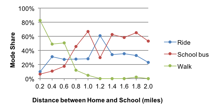
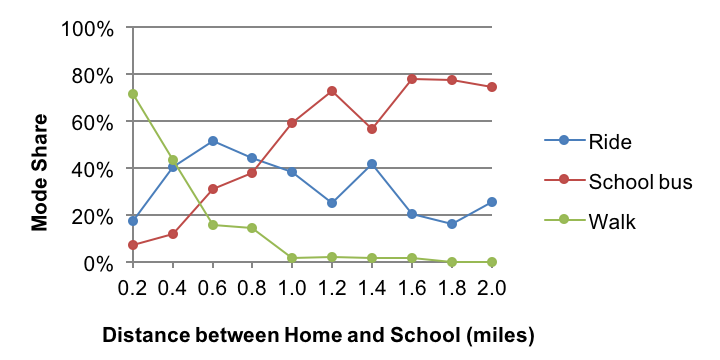
In both the central and non-central sector travel markets, walking was the mode of choice for short distance trips, with a walk mode share greater than 80 percent in the central sector and more than 70 percent elsewhere for distances of 0.2 miles or less. Students tended to walk farther in the central sector than in the rest of the region. For most distances of less than one mile, the walk mode share was larger in the central sector than in the non-central sector.
Outside the central sector, the school bus mode share generally increased as the distance between home and school increased. Generally, the opposite was seen with respect to the ride mode share, which peaked at more than 50 percent for students living between 0.4 and 0.6 miles of school. This may reflect limited availability of safe walking or bike routes or larger ride mode shares reflecting parents who drop students off at school on the way to work.
The mode shares and factors affecting mode choice are different for middle school students than for elementary school students, primarily because of differences in age and school bus policies. Middle school students are older, and therefore more likely than elementary school students to take transit by themselves. In addition, schools are not required to provide free transportation to middle school students, with the exception of students in regional school districts who live farther than 1.5 miles from school.
Transit was more competitive for middle school students in the central sector than in the rest of the region, which is consistent with the findings in the major school travel markets. As shown in Table 13, transit had a 17 percent mode share for middle school students in the central sector, but only a three percent mode share outside the central sector. However, almost half of the students outside the central sector rode a school bus. When the transit and school bus modes were combined, the total transit-related share of 50 percent outside the central sector was larger than the transit-related share of 42 percent in the central sector. The ride mode share was consistent between the travel markets, at 29 percent in the central sector and 31 percent in the other locations. Both middle school travel markets were transit-competitive when school buses were included in the definition of transit.
Table 15 shows the mode shares for households without a vehicle and households with at least one vehicle for middle school students who traveled to school in the central sector. Within this transit-competitive travel market, the number of vehicles in the household had a noticeable effect on the transit mode share. The transit mode share decreased from 22 percent in households without any vehicles to 15 percent in households with at least one vehicle. For comparison, the school bus mode share decreased by a much larger amount, from 51 percent in households without any vehicles to 15 percent in households with at least one vehicle.
Mode |
Percent |
Percent Households |
Bike |
2 |
4 |
Ride |
2 |
39 |
School bus |
51 |
15 |
Transit |
22 |
15 |
Walk |
23 |
27 |
Total |
100 |
100 |
Table 16 shows the mode shares for the high school travel markets. In the central sector, only 10 percent of students took a school bus, but 44 percent took transit, for a total transit-related share of 54 percent. Outside the central sector, 33 percent of students took a school bus, while only three percent took transit, for a total of 36 percent. Transit is competitive in the central sector, and school bus is competitive elsewhere. The auto-related share of students who drove or got a ride to school was 21 percent in the central sector and, as expected, a much larger 51 percent outside the central sector.
Mode |
Number of Students in Central Sector |
Number of Students Elsewhere |
Percent Share |
Percent Share Elsewhere |
Bike |
2,962 |
1,420 |
5 |
1 |
Drive |
1,067 |
17,384 |
2 |
13 |
Other |
191 |
924 |
0 |
1 |
Ride |
10,086 |
51,458 |
19 |
38 |
School bus |
5,519 |
44,291 |
10 |
33 |
Transit |
23,709 |
3,683 |
44 |
3 |
Walk |
10,357 |
16,946 |
19 |
12 |
Total |
53,891 |
136,106 |
100 |
100 |
This subsection analyzes factors that may affect mode choice for students in the high school travel markets. Both the central and non-central sector travel markets are transit-competitive when school buses are considered to be transit related.
One major difference affecting the mode choice of high school students and their younger primary school counterparts is the addition of the driving mode for students who have driver licenses. The legal driving age in Massachusetts is 16 years and six months, so the impact of driving eligibility on mode choice was explored by dividing the travel markets into students who were not eligible to get a license (ages 14-15) and students who were eligible to get a license (ages 17-18). This analysis excluded 16-year-old students because they may or may not have been eligible to get a license at the time of the survey. Table 17 shows the mode shares for these groups of students in each of the high school travel markets.
Within each travel market, the transit mode share was not negatively affected by the eligibility of older students to obtain driver licenses. The transit mode share for students in the central sector travel market was larger in the license-eligible group than in the license-ineligible group by 11 percent. Offsetting the increases in the transit and drive modes, the ride and school bus mode shares decreased, with the school bus mode share dropping to just one percent in the license-eligible group.
|
Percent License-Ineligible Students in Central Sector |
Percent License-Eligible Students in Central Sector |
Percent License-Ineligible Students Elsewhere |
Percent License-Eligible Students Elsewhere |
Bike |
6 |
8 |
2 |
0 |
Drive |
0 |
5 |
0 |
35 |
Other |
0 |
1 |
0 |
2 |
Ride |
23 |
16 |
42 |
26 |
School bus |
10 |
1 |
40 |
19 |
Transit |
41 |
52 |
3 |
2 |
Walk |
20 |
17 |
13 |
15 |
Total |
100 |
100 |
100 |
100 |
Note: License-ineligible groups are ages 14-15. License-eligible groups are ages 17-18.
It is apparent from the significant transit mode share and very small drive mode share (five percent) that driving was not a major competitor in the central sector high school travel market. This may be because most households did not have a vehicle available for the student to take to school. Efforts to increase the transit mode share in this market may be fruitful because transit is already an established mode, even among students who are eligible to obtain a license. However, transit use and walking already make up nearly 70 percent of the mode share, so the market for these modes may be saturated. In addition, very few students drove to school, so any mode shift from driving to transit would be small.
At between two and three percent, transit mode share for students outside the central sector was very small, but consistent between license-eligible and license-ineligible students. The drive mode share in the license-eligible group was 35 percent. The ride and school bus mode shares decrease when students are eligible to receive their license. Although driving eligibility did not seem to have an impact on the transit mode share, the transit mode shares were so low that the addition or improvement of transit services in this travel market may not be enough to cause a mode shift.
While the driving age was found not to have an effect on transit mode share in the high school travel market, the mode shares of students with and without driver licenses were also analyzed to understand how many license-eligible students actually have driver licenses and how many licensed students drive to school. At 60 percent in the central sector and 58 percent elsewhere, the response rate to the survey question about possessing a valid driver license was consistent. Some students did not respond because they were not asked the question based on their stated ages.
In the central sector, only 14 percent of students who answered the question had a license, and 23 percent of those who had a license drove to school. The results were quite different outside the central sector. Almost half, 45 percent, of the students who answered the question reported that they had a license, and of those, 49 percent drove to school. The higher rate of licensed drivers and larger drive mode share outside the central sector aligns with the mode shares in Table 17. It is interesting to note the low licensed driver rate in the central sector, which may reflect the greater density and resultant transit-oriented culture there.
Both the percentage of eligible students who had a license and the percentage of licensed students who drove to school vary significantly between the travel markets. These results are consistent with previous findings in the high school and other major school travel markets: school location, in relation to the central sector, has a very significant influence on transit mode share. While the licensed driver rate differed between the two locations, the transit mode share in each market did not decrease, indicating that the driving age and possession of a driver license do not affect transit mode share.
Table 18 shows the mode shares for college students in the central and non-central sector travel markets. Driving and transit were the primary modes used by college students in the Boston Region MPO area. In the central sector, the transit mode share of 56 percent was more than double the drive mode share of 26 percent. Outside the central sector, the mode shares were opposite and more polarized, with 76 percent of students driving and only nine percent taking transit to school. The walk mode had a five percent greater share of the market in the central sector than of the market outside the core area.
|
Number of Students in |
Number of Students Elsewhere |
Percent Share Central Sector |
Percent Share Elsewhere |
Bike |
3,322 |
564 |
2 |
1 |
Drive |
36,227 |
53,686 |
26 |
76 |
Other |
838 |
315 |
1 |
0 |
Ride |
4,941 |
5,292 |
4 |
7 |
School bus |
0 |
0 |
0 |
0 |
Transit |
77,795 |
6,545 |
56 |
9 |
Walk |
15,609 |
4,304 |
11 |
6 |
Total |
138,732 |
70,706 |
100 |
100 |
The regional travel demand model analyzes all commuter college trips together, but the travel survey results specified four types of colleges: technical/vocational school, community college, university, and graduate school. The college types have different characteristics that may affect mode choice, so the mode shares for each college type were analyzed within the two major college travel markets. Table 19 shows the mode shares by college type in the central sector, and Table 20 shows the mode shares by college type outside the central sector.
|
Vocational School |
Community College |
|
Graduate School |
Bike |
0 |
2 |
2 |
4 |
Drive |
15 |
18 |
27 |
32 |
Other |
4 |
0 |
0 |
1 |
Ride |
2 |
12 |
2 |
1 |
School bus |
0 |
0 |
0 |
0 |
Transit |
67 |
67 |
59 |
43 |
Walk |
12 |
1 |
9 |
19 |
Total |
100 |
100 |
100 |
100 |
|
Vocational School |
Community College |
|
Graduate School |
Bike |
0 |
0 |
0 |
4 |
Drive |
79 |
77 |
73 |
78 |
Other |
0 |
0 |
1 |
0 |
Ride |
15 |
12 |
4 |
6 |
School bus |
0 |
0 |
0 |
0 |
Transit |
7 |
8 |
12 |
7 |
Walk |
0 |
3 |
10 |
5 |
Total |
100 |
100 |
100 |
100 |
Within the central sector travel market, community college and technical/vocational school students had larger transit shares and smaller drive mode shares than those of university and graduate school students. In general, the mode shares were more consistent among college types outside the central sector than in the core region, where transit is denser but its attractiveness may be localized based on each school’s proximity to service.
The travel market of college students traveling to school in the central sector is transit-competitive and the transit mode share is larger than the drive mode share for the market as a whole. Transit also has a larger mode share than driving among those students living in households with at least one vehicle, indicating that students recognize the benefits of transit even when they have a choice between transit and auto modes. Shifting existing auto trips to transit may be more likely for this travel market than for others because transit is already attractive to a large percentage of these students.
This subsection examines the factors that affect mode choice for college students, with a focus on the central sector travel market. While transit may not be a feasible alternative outside the central sector, opportunities may exist to influence mode shift from driving to other healthy transportation modes (walking or biking) in these locations.
Table 21 shows the mode shares by income bracket in the central sector college-student travel market. The transit mode share is larger than the drive share in all of the income brackets, but there were no clear trends across all of the income brackets represented in the survey. The bike, other, and ride modes are not included in the table because they had overall shares of three percent or less.
Household Income |
Percent Drive |
Percent Transit |
Percent Walk |
Less than $25,000 |
18 |
58 |
14 |
$25,000 - $34,999 |
20 |
61 |
18 |
$35,000 - $49,999 |
9 |
76 |
9 |
$50,000 - $74,999 |
29 |
60 |
8 |
$75,000 - $99,999 |
29 |
46 |
18 |
$100,000 - $149,999 |
40 |
46 |
10 |
$150,000 or greater |
33 |
55 |
6 |
Note: Bike, other, and ride mode shares are not shown because they are very small.
The school’s proximity to transit, measured by the distance to the nearest rail station, has a significant effect on mode share. This metric is similar to the distance between work and transit, which staff found was correlated with the transit mode share for work commuting trips. Table 22 shows the mode shares by distance between school and transit for zero-vehicle households and households with at least one vehicle in the central sector college travel market.
Distance from School to Transit (miles) |
PercentZero Autos Drive |
Percent Zero Autos Transit |
Percent 1+ Autos Drive |
Percent 1+ Autos Transit |
Percent Total Drive |
Percent Total Transit |
Less than or equal to 0.25 |
0 |
72 |
25 |
59 |
21 |
61 |
0.26 - 0.50 |
2 |
72 |
44 |
46 |
35 |
51 |
0.51 - 0.75 |
0 |
16 |
44 |
37 |
37 |
34 |
0.76 - 1.00 |
N/A |
N/A |
54 |
46 |
54 |
46 |
N/A = not applicable.
As expected, the transit mode share decreased and the drive mode share increased as the distance from school to transit increased. Students attending colleges located within one-quarter mile of transit had a 61 percent transit mode share and 21 percent drive mode share. For colleges located between one-quarter mile and one-half mile from transit, 51 percent of students took transit and 35 percent drove to school.
The relationship between the proximity to transit and the drive and transit mode shares holds for households with at least one vehicle. Students living in these households had the option to take transit or drive, yet only 25 percent of those who attended school within one-quarter mile of transit drove to school. Within one-half mile, the drive and transit mode shares were closer to each other in households where both modes were available than in the overall travel market that includes households without a vehicle.
The 21 percent of students at schools within one-quarter mile of transit who drove to school present a potential opportunity to influence mode shift given the close proximity of their schools to transit. However, the distance between their homes and transit likely is also a factor in their mode choice.
Table 23 shows the drive mode shares by the distance from home to transit for those college students who attend schools in the central sector that are within one-quarter mile of transit. As shown in Table 23, approximately half (54 percent) of these drivers live within one mile of the nearest rail station. The percentage is larger for those who live in the central sector and smaller for those who live elsewhere in the region.
Distance from |
Percent |
Percent |
Percent Total |
Less than or equal to 1.00 |
80 |
39 |
54 |
1.01 - 2.00 |
20 |
13 |
16 |
Greater than 2.00 |
0 |
48 |
30 |
In comparison to the drive mode share table, Table 24 shows the transit mode shares by the distance from home to transit for the same travel market. As shown in the table, 51 percent of transit users whose school was within one-quarter mile of transit and whose home was outside the central sector live within one mile of the nearest rail station, and 23 percent live farther than two miles. The students who live farther than two miles from transit likely would choose drive-access transit, which may be a feasible alternative for those who currently drive to schools that are very close to transit.
Distance from |
Percent |
Percent |
Percent Total |
Less than or equal to 1.00 |
93 |
51 |
79 |
1.01 - 2.00 |
7 |
26 |
13 |
Greater than 2.00 |
0 |
23 |
8 |
Importantly, the distribution of the distance between school and transit differs between the two college travel markets. In the central sector, 93 percent of students attended a college located within one-half mile of transit. By comparison, outside the central sector, only 27 percent of students attended a college located within one-half mile of transit. This is consistent with the main finding that transit has a larger mode share for college trips in the central sector than in the rest of the region. The central sector has a denser transit network, leading to generally shorter distances between schools and rail stations, and resulting in a larger transit mode share.
Opportunities exist to shift mode choice from auto to transit or school bus in all of the markets in the central sector and the primary and high school markets outside the central sector. As shown in the previous section, only the high school and college student travel markets in the central sector are truly transit-competitive. However, both of the primary school travel markets and the high school travel market outside of the central sector have competitive shares of school bus trips compared to the ride mode share.
This section describes specific recommendations to increase the transit mode share for school-related trips. Importantly, the strategies to increase the transit mode share for work trips discussed in Section 4 broadly relate to school trips as well. The strategies are particularly relevant for the college travel markets, where school bus is not a mode choice and where there is a clear distinction between the transit-competitive central sector and the non-transit competitive portion of the region. However, the recommendations in this section are tailored to the distinctive characteristics and needs of students at the primary school, high school, and college levels.
The proximity of school to transit is an important factor affecting mode share, particularly in the transit-competitive college travel market in the central sector. This factor has a similar effect on the drive and transit mode shares of school trips as that of the distance between work and transit on commuter trips described in Section 3. Transit projects that serve large institutions such as universities have the potential to influence a mode shift because of the strong effect of the distance between school and transit on the transit mode share.
Improving the proximity of a school to transit service affects all of the students attending the school, regardless of the proximity of their homes to transit, because students who currently drive to school could shift to transit. College students are more likely to live close to transit in the central sector than in the rest of the region, but even outside the core area, transit is a feasible mode for students whose school is located in close proximity to transit. College students also may be more transient than non-student workers, so they might be more likely to choose their home locations based on the location of their schools and the transit network that serves them.
In the central sector travel markets, transit mode shares generally increased as student age increased, from five percent in the non-transit-competitive elementary school travel market to 56 percent in the highly competitive college market. Outreach to students may be beneficial in some school travel markets where transit is already competitive. This subsection describes potential outreach opportunities for middle school and college students.
Transit was competitive in the central sector middle school travel market, which had a 17 percent transit mode share and 29 percent ride mode share. However, students also rode the school bus (25 percent) and walked (26 percent) more frequently than they took transit. Young middle school students may not be as accustomed to taking transit by themselves as older high school and college students. Providing outreach and information about how to use the transit system may help increase the transit mode share for middle school students. However, transit should be promoted along with school bus riding and walking, because the goal is not to shift students to transit who already take the school bus or walk.
Outreach to promote transit also may be helpful in the central sector college student travel market. Although the transit mode share was more than double the drive mode share in this market segment, 26 percent of students drove to school. Thus, there are additional opportunities to increase transit mode share among students of schools with existing high transit mode shares. Better publicizing of transit options for incoming students, particularly before they have chosen where to live, may help increase transit mode share at these schools.
The MBTA Youth Pass pilot program and upcoming implementation of a permanent Youth Pass program also present opportunities to increase the transit mode share for school trips. Ultimately, a major purpose of the pass program is to increase the number of students who qualify for reduced fares. The program may reach students whose schools currently do not offer such passes. Furthermore, publicizing these programs may increase awareness about transit as a viable mode for students in general.
One potential for mode shift away from the auto is to increase the school bus mode share for primary school students. At least 30 percent of elementary school students got a ride to school in both travel markets, even though many lived close to school or had access to free school bus transportation. A similar percentage of middle school students got a ride to school as well.
The school bus mode is an important and competitive mode for elementary and middle school students in both the central sector and non-central sector travel markets. Opportunities to increase school bus mode share vary between elementary and middle school students because there are different school bus policies for each.
School buses are provided free of charge to elementary school students living more than two miles from school. In both the central sector and the rest of the region, school-bus ridership represents a larger mode share beyond the two-mile threshold than within it. A reduction in school bus fees may encourage a mode shift by incentivizing students who get rides to take the school bus. A change in the free school bus policy, such as reducing the threshold from two miles to one mile, also may increase the school bus mode share and decrease the ride mode share.
The school bus mode was competitive in the central sector middle school travel market and highly competitive in the rest of the region, even though most middle school students must pay for bus service. In both travel markets, the school bus mode share decreased as household income increased. The fee may not be a major barrier to students taking the school bus, but providing incentives for students to take the school bus to schools outside the central sector instead of getting a ride to school may help influence a mode shift.
In addition to transit and school bus modes, walking and biking are non-auto options that, from a mode-shift perspective, are more desirable than driving or getting a ride to school. Encouraging these active transportation modes also aligns with MassDOT’s Healthy Transportation Compact and the statewide goal of tripling the distance traveled by transit, walking, and biking by 2030.
In addition to transit and school bus modes, walking and biking are non-auto options that, from a mode-shift perspective, are more desirable than driving or getting a ride to school. Encouraging these active transportation modes also aligns with the Massachuetts Department of Transportation’s Healthy Transportation Compact and the statewide goal of tripling the distance traveled by transit, walking, and biking by 2030.
These healthy transportation modes may be particularly attractive and have greater potential for elementary school students who live close to school and do not receive free school bus service. Twenty-nine percent of these students in the central sector travel market got a ride and 36 percent outside the central sector got a ride.
The Massachusetts Safe Routes to School program4 was piloted in 2000, in Arlington,5 and launched across the state in 2006. The program now has more than 500 partner schools, and as of 2012 had reached 35 percent of students in kindergarten through eighth grade. Safe Routes to School programs encourage elementary and middle school students to walk and bike to school through efforts such as improving access to schools and teaching children about bicycle safety, with the overall goal of improving child health and well-being. Implementing Safe Routes to School tools, and funding additional such programs, could reduce the ride mode share and shift those students to walking and biking modes, while improving student well-being. While Safe Routes to School programs are not designed for transit, increasing the healthy transportation mode shares in the primary school travel markets is much more likely than increasing the transit share.
4 Massachusetts Department of Transportation, “Massachusetts Safe Routes to School Program Celebrates Exclusive Milestone of 500 School Partners,” last modified September 20, 2012, www.massdot.state.ma.us/main/tabid/1075/ctl/detail/mid/2937/itemid/214/
Massachusetts-Safe-Routes-to-School-Program-Celebrates-Exclusive-Milestone-of-500-School-Partners.aspx.
5 National Center for Safe Routes to School, “How did Safe Routes to School begin?” http://www.saferoutesinfo.org/program-tools/how-did-safe-routes-school-begin.
The MPO’s regional travel demand model is used to predict future transportation conditions based on different transportation-investment and demographic-trend scenarios. The model can estimate the number of trips that will be made on a typical weekday or weekend day, where the trips will originate and terminate, what modes will be used, and what routes will be taken.
This study relates to the mode-choice step of the model, which estimates the number of people who would chose each mode and the resulting mode shares for different types of trips. Trips are assigned to the mode that would provide the greatest utility, or satisfaction, for travelers based on variables such as monetary cost, travel time, and other measures of convenience. The determination of utility is discussed in the next section.
The travel demand model contains mode-choice models that predict the mode of travel people would likely choose based on their trip purpose and considering their varied values of time and decision-making processes. The models for home-based work and home-based school trips are pertinent to the mode shift analysis in this report. All home-based work trips were modeled together, while home-based school trips were grouped into three categories based on student age.
The 2011-MTS data are key inputs to the model that shed light on traveler behavior and preferences, along with other data that represent the characteristics of different modes in the transportation system. Geographic data such as population, employment, and parking costs are also developed and incorporated in the mode-choice models.
The model quantifies the effects of the various factors that influence mode choice for base-year (or current) conditions in order to predict the mode share under future scenarios. Analyses from the mode-choice models should align with the mode-choice findings in this study because the models are also based on data from the 2011-MTS. The model also provides insights into the relative importance of different factors affecting mode choice, as described in the next section.
People consider different factors when choosing modes depending on their trip purposes. For example, a trip from home to work may be especially time-sensitive, so a mode with a longer travel time may be less desirable. A recreational trip may be less time-sensitive, so the travel time may not have as large an impact on mode choice as it would for the work trip.
The weights of these factors are captured in the mode-choice models by constant values, called coefficients, which are multiplied by the data for each variable to determine the overall utility of choosing each mode relative to the others for a given trip. The mode-choice models determine different coefficients for each variable and trip type based on data about traveler behavior, including the 2011-MTS, and data about the transportation system and land use characteristics. , including the 2011-MTS.
This section describes the coefficients of the factors for the mode-choice models for home-based work and home-based school trips, comparing the coefficients for the factors that were included in the various model specifications. By examining the coefficients, we can understand which factors contribute to mode choice and use this information to influence a mode shift.
Level-of-service variables refer to characteristics of a trip that vary by mode, such as travel time and cost. These variables capture the cost of choosing a given mode, measured by the time and money spent for a particular trip. Table 25 shows the level-of-service variables and their coefficients for the mode-choice models that are relevant to this study.
Level-of-Service Variable |
Work |
School |
School |
School |
In-vehicle travel time |
-0.020 |
-0.011 |
-0.016 |
-0.018 |
Out-of-vehicle travel time a |
-0.060 |
-0.034 |
-0.047 |
-0.054 |
Terminal time b |
-0.269 |
-0.150 |
-0.366 |
-0.083 |
Cost |
-0.111 |
-0.146 |
-0.147 |
-0.150 |
a Out-of-vehicle time does not apply to the drive mode.
b Terminal time does not apply to the walk or walk-access transit modes.
Note: Coefficients are for drive, ride, and transit modes.
All of the model specifications include variables for cost, in-vehicle travel time, and a measure of out-of-vehicle travel time, such as terminal time. Terminal time refers to the out-of-vehicle travel time for auto modes and the out-of-vehicle travel time at only the origin end of the trip for drive-access transit modes.
The coefficients for the travel time and cost variables are negative in all of the model specifications, indicating that modes that take less time or cost less money are more desirable than modes that take more time or cost more money. The components of out-of-vehicle travel time, such as access time, wait time, and transfer time, are not separately specified in the model, so their individual importance and relative effects cannot be determined.
The values of the coefficients, and thus the weights they represent, may be compared between trip types by reading across the rows shown in Table 25. The coefficients for in-vehicle travel time become more negative as the age of the students making a school-related trip increases, indicating that older students have a greater value of time than do younger students. Work trips have the most negative in-vehicle travel time coefficient, indicating the greatest value of time.
While the travel-time coefficients are smaller for the school trip categories than for the work trips, the coefficients for cost are larger for students than for commuters. This suggests that people traveling to work are more sensitive to time, while students traveling to school are more sensitive to cost.
One may understand the relative importance of the coefficients in each mode choice model by comparing down each column. The values of the coefficients for out-of-vehicle travel time are set to be three times the values of the coefficients for in-vehicle travel time for each trip purpose, based on Federal Transit Administration guidelines and calibration using survey data. This is consistent with the finding that the distance from work or school to the nearest transit station affects mode choice, as access time is part of out-of-vehicle travel time, which is weighted heavily in the model.
The coefficients for terminal time are much more negative than those for in-vehicle travel time and out-of-vehicle travel time, meaning that terminal time is valued more highly than other travel time for the drive-access transit and drive modes. This implies that travelers who choose to drive, either for their entire trip or to a transit facility, are less tolerant of out-of-vehicle time than travelers who do not drive for any part of their trip.
In addition to level-of-service variables, the mode-choice models contain geographic variables that relate to characteristics of the trip that are not dependent on the transportation mode. For example, the variables of employment density and straight-line distance between the origin and destination are the same for a given trip regardless of the mode. The geographic variables related to density and distance between home, work, school, and transit are particularly pertinent to the earlier discussion in this report.
The mode-choice models for each trip purpose were refined using the 2011-MTS data to include the variables and coefficients that best matched the survey results. Most of the geographic variables are only included in the mode-choice models for one or two trip purposes, and some of the variables are only included for a particular mode. Some variables that are included in different models are very similar, so the geographic variables are discussed by topic in the subsections below.
The mode-choice models for home-based work and college-aged home-based school trips include an employment-density variable. Employment density is calculated for the destination end of these trips as a proxy for the auto parking conditions. The coefficient for the employment-density variable is positive for the walk, walk-access transit, and drive-access transit modes and negative when applied to the drive modes. This is consistent with the findings in Section 3 that transit is more attractive in high-density locations.
The mode-choice models for primary and high school students include a variable for population density. Population density is calculated at the origin of the trip, indicating that home location is important; however, schools are generally closely related to home locations at the primary and high school levels.
As expected, population density is positively correlated with the utility of the walk and walk-access transit modes. This is consistent with the mode shares discussed in Section 5, as the primary and high school travel markets in the higher-density central sector had larger walk and transit mode shares than their counterparts elsewhere.
As shown in Section 3, the proximity of work to transit is an important factor in the transit and drive mode shares for work-related trips. The mode-choice model for work trips includes a “walk-access fraction” variable that measures the amount of a geographic zone that is within one mile of transit stops. The values of the variable range from zero (no part of the zone is within one mile of transit) to one (the entire zone is within one mile of transit).
The coefficient of the walk-access fraction variable has a value of 1.84 for walk-access transit modes and 1.46 for drive-access transit modes. The larger coefficient for walk-access transit modes reflects the greater importance of proximity to transit than for drive-access transit modes. The survey responses do not distinguish between walk-access and drive-access transit, but the range of distances from home to transit indicates a mixture of access modes in the results.
Although the proximity of school to transit was found to be an important factor in the central-sector college-student travel market, the mode-choice model for college-aged school trips does not include the walk-access fraction variable. Many variables were tested in different variations of the mode-choice models, but only the combination of factors that best captured the survey results were included in the final model specifications.
The models for work trips and college-aged school trips include a “pedestrian environmental variable” that captures the ease and comfort of walking in a given area. The variable is based on the proportion of roadways that include sidewalks, the proportion of roadways that are designated as truck routes, and several factors that affect pedestrian level of service, such as the width of the outside lane of traffic and the average speed of vehicles on the roadway.
A smaller value for the pedestrian environmental variable indicates a better walking environment. The variable is included in the utility for the walk, bike, and walk-access transit modes in the mode-choice models for work- and college-aged school trips, as well as the drive-access transit modes in the school model. The coefficient of the variable is negative in both models, reflecting the inverse relationship between the pedestrian environmental variable and the attractiveness of the non-auto modes.
The pedestrian environmental variable is an example of a factor that affects mode choice but is not readily apparent in the 2011-MTS results. The model captures the relationship between the pedestrian environment and mode choice by combining the 2011-MTS data with transportation system characteristics. The pedestrian environmental variable can help explain variation in mode shares where other measures such as density and proximity to transit are similar.
The mode-choice model for primary school-aged trips includes a variable for the distance between the origin and destination of the trip. A coefficient of -0.0426 is applied to the distance for the walk mode, and a coefficient of -0.0280 is applied to the variable for the bike mode. The coefficients are both negative because a longer distance would mean a decrease in the attractiveness of walking and biking. The relative magnitude of the coefficients indicates that the distance affects walk trips more than bike trips.
The mode choice model for college-aged school trips uses a similar variable to capture the relationship between trip distance and the utility of the walk mode. The variable has a value of one if the distance between home and school is within one mile, and a value of zero otherwise, indicating that walking is more attractive within one mile than beyond that distance. While the distance people are willing to walk varies by individual, this variable generally captures the relationship between short distances and the attractiveness of the walk mode.
The analysis in Sections 3 and 5 found that transit mode share is strongly affected by whether a household has at least one vehicle. Even in the school travel markets where transit was competitive, the transit mode share was larger for households without any vehicles, as expected, because students in those households did not have the option to drive or get a ride to school. There were no clear trends between mode choice and other demographic factors such as household income and education level.
Similarly, the only socioeconomic variable included in the mode-choice models is the number of vehicles per worker. The variable was included in the mode-choice models for work trips and college-aged school trips. A coefficient of 1.25 was applied to the number of vehicles per worker for the drive-alone mode in the work trip model, and a coefficient of 1.59 was used for the drive-access transit modes in the same model. In the school-trip model, a coefficient of 1.52 was applied to the number of vehicles per worker for the drive-alone mode and a coefficient of 2.39 was used for the shared-ride mode.
The positive coefficients in the mode-choice models indicate that the number of vehicles per worker is directly correlated with the attractiveness of the auto-related modes. The inclusion of this variable in the model specifications supports the findings from the survey that access to a vehicle has a strong effect on mode choice. The coefficients also suggest that the number of vehicles per worker is important, in addition to whether the household has any vehicles.
The recommendations in Section 4 describe strategies for improving transit service to influence a mode shift for work trips. The opportunities presented in Section 5 suggest additional ways to influence a mode shift specific to school trips. The findings from the model are consistent with these results, and they provide detailed insights about factors that affect mode choice.
We mean for the opportunities described in this section to supplement and combine with the strategies and recommendations cited earlier. It is important to consider the role of density and proximity to transit, as shown in the model results and previous findings, when applying these recommendations. Density and proximity to transit affect the level of effort needed to influence a shift to transit, but the opportunities described here still can be applied to most locations.
It is clear that reducing transit travel time would increase the attractiveness of the transit mode for a given trip. There are many components of travel time for a transit trip in particular, and the model coefficients can inform the priorities about how to best increase the utility of the transit mode in this way.
Out-of-vehicle travel time is valued at three times in-vehicle travel time in all of the mode-choice models. Therefore, reducing out-of-vehicle travel time has a much larger effect on satisfaction or utility than reducing in-vehicle travel time by the same amount of time. Some aspects of out-of-vehicle travel time are mostly outside the transit service’s control, such as access and egress times. However, improved service frequency can reduce transfer and wait times, which also are components of out-of-vehicle travel time.
While in-vehicle travel time is not valued as highly as out-of-vehicle travel time, reducing in-vehicle time still increases the attractiveness of a given mode. In each model, in-vehicle travel time has the same coefficient for the drive, ride, and transit modes. This suggests that an increase in the auto travel time would have the same effect on the relative utility of the modes as a decrease in the transit travel time by the same amount.
Increasing transit frequency reduces wait times, which contribute to the out-of-vehicle travel times. In particular, transit frequency affects the wait times for users making transfers or users who arrive at a stop or station without checking a schedule first. Users may be able to reduce their wait times for flexible trips by planning their arrival to a stop or station based on real-time information, but transit frequency is still an important factor that affects mode choice.
Transit frequency is very useful when making predictions about the mode-choice process, as users consider the frequency of service before selecting a mode. The availability of high-frequency service makes transit more attractive because it provides more flexibility and options for travel. Providing high-frequency service is an opportunity to influence a mode shift, and emphasizing these services through branding and marketing should be considered in order to maximize the potential benefit.
The mode-choice models capture the effect of cost, which is not explicitly included in the 2011-MTS data. The coefficient of the cost variable is the same for all modes in a given mode-choice model, except for the no-cost non-motorized modes. This means that a dollar spent toward a transit fare is valued the same as a dollar spent toward auto costs such as parking, and the costs can be directly compared across modes.
The variables in the mode-choice models are considered relative to each mode; changing the cost and attractiveness of transit can be achieved by increasing the price of driving as well as by decreasing transit fares. The costs for each auto mode in the model are divided by the number of occupants, so the carpool modes have a greater utility than driving alone when considering only the cost variable, and changes in cost affect the drive-alone mode more than the carpool modes.
The mode-choice models can be used to estimate the effect of adjusting the cost of a given mode relative to changing other variables. For example, a dollar increase in cost changes the utility of work trips by -0.111, while a minute increase in out-of-vehicle travel time changes the utility by -0.0599. The relationship between the coefficients tells us about the value of time assumed in the model based on the 2011-MTS dataset and can inform potential opportunities for mode shifts.
As seen in the 2011-MTS and model analysis, walkability is a factor in the mode choice decision that benefits transit as well as non-motorized modes. Some aspects of walkability that are included in the models have already been discussed in this report. For example, the distance between the origin and destination of a trip that is included in the school-trip model for the youngest-aged students also was analyzed for primary school trips in Section 5.
One factor included in the models but not in the 2011-MTS dataset is the pedestrian environmental variable, which measures how conducive the physical surroundings are to walking. Non-auto modes are more attractive in locations with favorable pedestrian environmental values. The variable is included only in the mode-choice models for work and college-aged school trips, but an improved walkable space would benefit all users regardless of trip purpose.
It is important to consider the pedestrian environment in addition to land use and density when trying to influence a mode shift away from auto-related modes. Because proximity to transit is another key factor in mode choice, focusing efforts on improving the pedestrian environment in locations near transit may be most beneficial. Conversely, locations that are not as close to transit may benefit from an improved pedestrian environment, which potentially could compensate for the longer walking distance to transit.
The goal of this study was to develop quantitative information from the 2011-MTS and related sources that can inform planning efforts with the objective of increasing transit’s share of regional travel. We performed and presented our analysis in a set of distinct steps:
In the 2011-MTS, 2,117,200 workers reported that they commuted to work either from a residence or to a workplace in the Boston Region MPO travel demand model area.
The model region and adjoining areas were divided into eight distinct sectors. Then six commuting submarkets were defined based on patterns connecting homes and workplaces between the eight sectors.
Of the 2,117,200 commuters, 1,503,400 reported that they drove to work, and 300,100 reported using transit despite living in a household with an auto. Driving and transit were in head-to-head competition for these 1,803,500 commutes as the distance of the commutes were generally too far for walking.
In only three of the submarkets were the fraction of commuters who chose transit higher than two percent. In these three submarkets, 667,200 commuters either drove or chose transit, with transit taking a 43 percent head-to-head share (285,600 commuters chose transit).
For transit-competitive commutes, distances from home to transit, work to transit, and density at the work location were calculated. These three factors were shown to influence mode choice in the 667,200 transit-competitive commutes.
For each of the three geographical factors cited above, staff calculated transit shares—based on distances between work and transit, and home and transit—which produced results showing that transit share depends on conditions at both ends of the commute.
Head-to-head transit shares were calculated based on income and education. No meaningful mode-choice preferences were observed.
Using implications derived from the survey, staff considered three strategies:
Calculations of average commute distances by submarket revealed that mode choice did not depend on commute distance. However, commute distance clearly had planning implications, as discussed below.
During this analysis, a number of planning implications became apparent.
In two of the six submarkets, transit mode share is strong, and in three submarkets, it is very weak. Large increases in the weak submarkets will not dramatically change region-wide mode share. Where transit mode share is strong, transit already has captured the customers where its advantages are greatest.
A new or expanded transit service may not win a significant number of commuters in any individual commuting submarket. However, many transit services can be configured to serve several commuting submarkets simultaneously, and the combined new ridership may be significant.
Planning efforts for new transit services and real-estate developments carefully scrutinize the conditions at one end of what will be numerous commutes. The ultimate mode choices will depend on conditions at the distant ends of the commutes, factors that generally cannot be controlled or even known.
A straightforward strategy to increase transit’s share of commuting is to facilitate existing economic and land-use trends that locate new jobs and housing in proximity to transit services serving transit’s stronger submarkets.
Service deterioration or elimination can meaningfully decrease transit’s mode share. To take advantage of positive land-use trends, transit service must not deteriorate.
While transit and driving are equally effective in covering commuting distances, the challenges of using these modes include accessing transit at the trip endpoints and the availability of parking at the work end. Inspection of socioeconomic variables suggests that the region’s commuters are remarkably similar in their choices regarding driving and taking transit.
The congestion and environmental impacts of commuting are roughly proportional to the commute distance. Estimated commute lengths should inform mode-shift policy development.
This study identified major school travel markets by school level and geographic location relative to the central sector, using data from the 2011-MTS. The 2011-MTS represented approximately 768,000 household students, almost half of whom were in primary school, with the remaining students approximately split between high school and college.
The existing mode shares differ noticeably among the school travel markets.
Transit had a mode share of only nine percent in the central sector, but transit usage was greater within the submarket of older middle school students. Travel by school bus was a critical transit-like mode for primary school students, particularly outside the central sector where transit is less available.
Transit was very competitive and had the largest share of all the modes in the central sector, with 44 percent of high school students taking transit to school. Outside the central sector, most students got a ride or took the school bus, while the transit mode share was only three percent.
In the central sector, the transit mode share was 56 percent and the drive modes share was 26 percent. Outside the central sector, the transit mode share was nine percent and the drive mode share was 76 percent. Transit was very competitive in the central sector, but driving was the only competitive mode in the college travel market outside the central sector.
The 2011-MTS data also provided insights into the factors affecting mode choice and implications for a mode shift in the school travel markets.
The most notable factor affecting transit mode share in the school travel markets was the geographic area in which the school was located because dense areas generally have more transit service than less-dense locations. In the dense central sector, nine percent of primary school, 44 percent of high school, and 56 percent of college students commuted by transit. By comparison, only two percent of primary school, three percent of high school, and nine percent of college students who attend school outside the central sector commuted by transit.
As expected, the transit mode share decreased and the drive mode share increased as the distance between school and transit increased. The proximity of school to transit was also related to density, as 93 percent of students in the central-sector travel market attended a college located within one-half mile of transit, compared to only 27 percent of students in the non-central-sector market.
The largest school bus mode share occurs in the non-central-sector primary school travel market, with 44 percent of students riding a school bus. The mode is also competitive in the central-sector primary and non-central sector high school travel markets, with approximately one-third of the mode share in each market.
In the transit-competitive central-sector high school travel market, the transit mode share was larger among students of driving age than among their younger peers. The mode shares in the high school travel markets are influenced much more by density and location than by age and possession of a driver license.
Most socioeconomic factors do not have a strong influence on mode shares in the school travel markets, except household vehicle ownership, which has a clear effect on mode share, as expected. Household income has an effect on the ride and school bus mode shares in the lowest and highest income brackets of the primary school central-sector travel market, which may be related to vehicle ownership as well.
Considering the unique nature of school trips, availability of other modes such as travel by school bus, and the young age of some students, this study identified opportunities to influence mode shift specifically in the school-travel markets.
The regional travel demand model predicts future transportation conditions based on different transportation-investment and demographic-trend scenarios. Within the travel demand model, specific mode choice models have been developed that capture and quantify the effects of different factors on mode choice by trip purpose. The mode choice models use data from the 2011-MTS as well as geographic and transportation system data.
The findings from the mode choice models agree with or supplement the 2011-MTS analysis results.
The value of time differs by trip purpose, with work trips having larger values than school trips. Out-of-vehicle travel time is set at three times in-vehicle travel time in the models, capturing the greater dissatisfaction with wait time and transfers.
All of the mode choice models include either an employment or population density variable that is positively correlated with the transit and walk modes. The proximity to transit is represented in the work trips model using a variable that measures the amount of the model zone that is within one mile of transit stops.
While the 2011-MTS dataset provides the distances between home, work, school, and transit, it does not explicitly include characteristics of the built environment. The mode choice models for work and college-aged school trips include a pedestrian environmental variable that captures these factors that affect walkability.
The opportunities for a mode shift to transit include decreasing transit travel time, increasing transit frequency, adjusting the relative costs of the modes, and improving the pedestrian environment.
The resources in the 2011-MTS provide a very complete picture of respondents’ commuting situations at the point that they chose their commuting modes. The geographical implications of proximity and density are quite clear and measurable. Implicit in a commuter’s mode choice is their willingness pay the cost to complete the commute via the chosen mode.
However, we cannot determine directly from the 2011-MTS what choice the commuter might have made if the prices were different. In further investigations of mode preferences in the Boston region planners clearly would want to estimate price sensitivity and pricing strategies, and these efforts could be informed by the analytical structure and geographical findings of this study.
It would be convenient to be able to directly apply information on transit modes shares based on geographical factors, such as shown in Figure 3, to a local residential or employment center, and develop a quick mode-share estimate. Unfortunately, without information about the other end of respondents’ commutes, we cannot utilize those analytical resources. However, there are instances where major local employers have relocated or considered relocating. In these cases, their personnel departments could perform a mode-shift estimation under the relocation scenarios. In fact, any regional entity willing to undertake a site-specific survey could use this approach.
It is possible, however, to start using the results of this study now. Major efforts to expand and improve transit are always being considered at some level, often informed by data from the Boston Region MPO’s travel demand model set. It also would be valuable to view these projects from the perspective of this study and consider the following: What are the markets served? What are their sizes? Can the outer ends of the commutes be anticipated in some manner? Given the challenges of introducing or successfully expanding a transit service, this new survey-based assessment could provide important insights when considering proposals for transit.